
Using Historic Stock Price Data in a Google Sheet
There are many great ways to analyze investments - particularly public company stocks - using the internet today. Yahoo Finance and Google Finance being the most easily found and used - but also MarketWatch, MSN and practically every broker and mutual fund site like Schwab and Fidelity when you have an account there - all provide loads of data, news and analysis.
Sometimes, those internet sources still don’t provide exactly what I want - which is often just a simple spreadsheet of historic price data on a particular stock.
A spreadsheet gives me flexibility to analyze the data, chart it, add hypothetical trades (yes, fake trades so I don’t actually lose money ;) and use it in other contexts by simply copying and pasting.
While some of the internet tools give me the ability to “export” stock data into a spreadsheet format (CSV or XLSX), that creates more work - saving the data, importing it into a spreadsheet, getting the formats right. I like to use a more direct method of getting the data into a spreadsheet, a Google Sheet in particular - and that is the GOOGLEFINANCE() Function. Even if you’re not a Spreadsheet superhero yet, and perhaps not comfortable yet with spreadsheet formulas, you can easily learn to use the Google Finance function - especially using the simple instructions in this post and the Google Sheet template I provide.
The Google Finance Function
Most Spreadsheet formulas use data from within the spreadsheet you are working in - and sometimes take data from other spreadsheets. The Google Finance function is unique in that it obtains data from a completely separate source of historic stock price data. But like any formula, it will require some inputs that you must provide. When using any spreadsheet formula, it’s important to understand those inputs, which gives you an idea of the options you have when you use the formula. The other special characteristic of this Google Finance function is that it will return data into more than the one cell where the formula is entered. It will return a whole table of data - one or more rows, one or more columns - in many cases. It will warn you if that returned data would have overwritten other data in your sheet.
The Google Finance function inputs are described in full in the Google Sheets help page. I’ll explain here the set of options that provides a simple history of stock price and other data - and won’t cover the many more options when requesting simply current data on a stock. If you are knowledgable about stock investing, I suggest you look more at that help page to see the extensive set of data you can get for current data when only retrieving one data attribute at a time. You can also use my other stock tracker spreadsheet template to go deeper on using current AND historic data in a format which lets you analyze the performance of hypothetical buy trades.
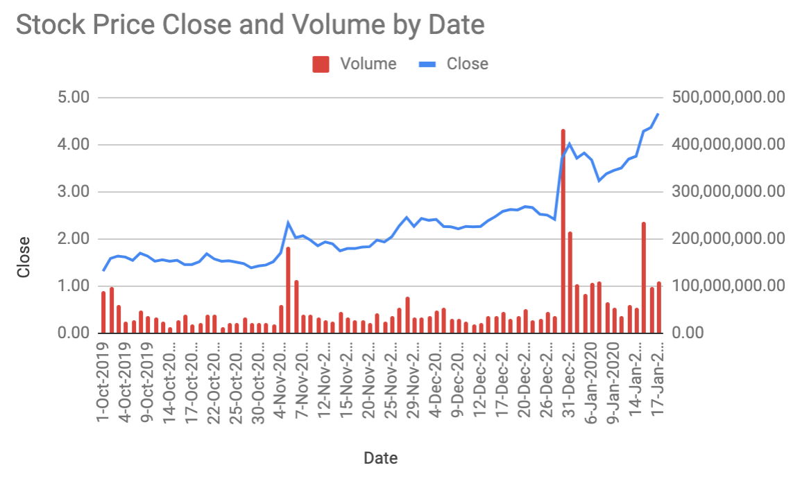
Once you have historical data, it’s also easy to chart it in a spreadsheet…
Getting Started
The format of the Google Finance function, used in a cell formula, is simply
=GoogleFinance(ticker, *attribute, *start-date, *end-date, *interval)
The asterisked inputs are optional, but we’ll focus on those, since that’s how you get historical price data. BTW, When you start the contents of any spreadsheet cell with an “=”, the sheet expects a formula.
ticker: This is the stock ticker of the stock you are seeking data about - and is the only REQUIRED input. If you only give ticker and nothing else, you’ll get back CURRENT price and volume data. Examples are TSLA for Tesla, GOOG for Google, F for Ford, Inc.
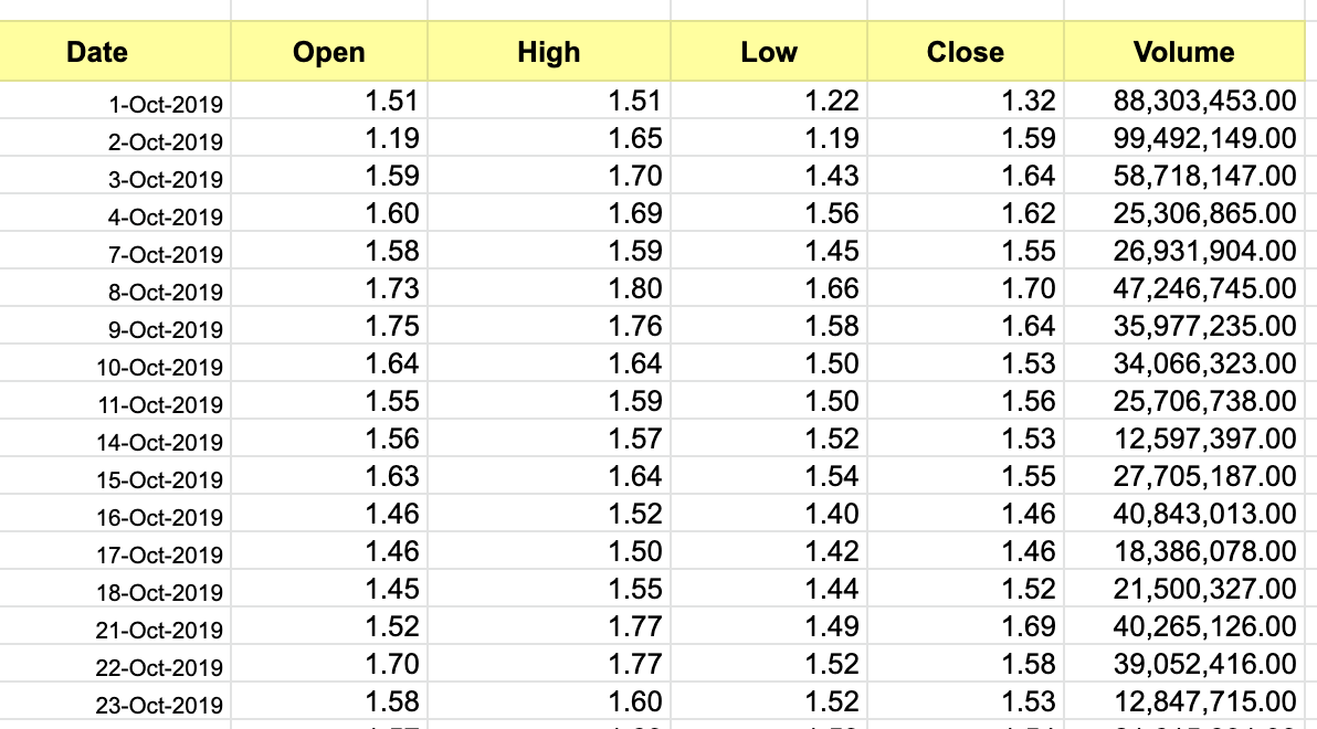
attribute: This is a choice of a specific data point, such as “OPEN”, “CLOSE”, “HIGH”, or more - or using the word “ALL” will return a whole set of date, open, high, low, close and volume (see help page for all options of specific attributes you can request - which is much larger when only requesting current data and not historic).
start-date: This is the beginning date of the historic data you are requesting.
end-date: This is the end date of the period for which you are requesting historic data.
interval: This gives you the ability to request either “daily” or “weekly” data (using those words, or the numbers 1 or 7 also work).
That’s pretty simple. Let’s look at one simple example:
=googlefinance( "tsla" , "all" , "1/1/2020" , "1/30/2020" , "daily" )
That example will return a table of data - 17 rows by 6 columns - of data for the stock of Tesla, Inc. The 17 rows represent one row for each BUSINESS DAY when the stock was traded during the period of Jan 1 through Jan 30, 2020 - and one row at the top with column headers. The 6 columns represent the data - date, open, high, low, close and volume.
Typing in that formula is not hard - but it’s not something you want to do every time you want data. The easier way to use formulas like this is to put the inputs to the formula in other cells, so you can easily change those inputs without changing the actual formula. So, in the sample spreadsheet I will provide you, my formula looks more like this:
=googlefinance( B5 , B6 , E5 , E6 , E7)
Those “CELL REFERENCES” above - like B5 - refers to the cells where the inputs will be in the spreadsheet. This method lets us change the value in B5, for example, to change the stock for which the data will be returned - or E7 to change whether the data returned is Daily or Weekly.
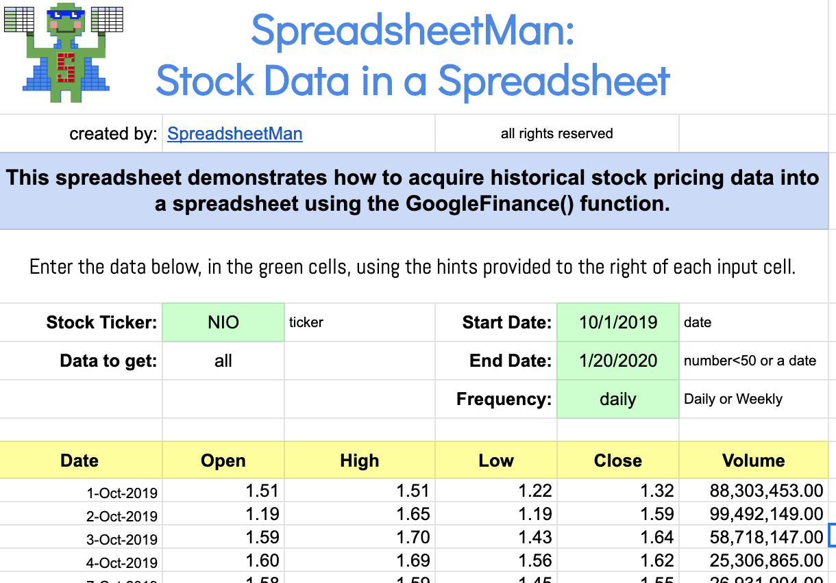
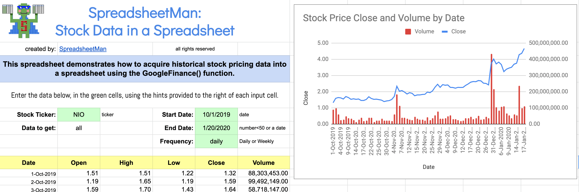
Google Sheets Template Using the Google Finance Funtion
Below is a screen shot image of the sample spreadsheet - and below that a link where you can request access so you can get your own copy.
Here is a link to get access to the free version of this Google spreadsheet!
If you have any questions or follow up posts you’d like to see, use the contact page link below!